BESS, deep learning simulations: decrease in wholesale price variability

As an energy expert embedded in utility operations, Leo uses deep learning and machine learning codes for analysis and forecasting to analyze and simulate market scenarios and optimize portfolio management strategies. In his most recent analysis, Leo used deep learning techniques to simulate PUN trends concerning the installation of utility-scale batteries. The PUN (Italian acronym for Prezzo Unico Nazionale, “National Single Price”) – the wholesale reference price of electricity purchased on the Borsa Elettrica Italiana market (IPEX – Italian Power Exchange) – represents the national weighted average of the zonal sales prices of electricity for each hour and for each day.

Graphs of electricity demand in power grids, look a bit like a duck or a camel (called the camel-backed curve here), with high points in the morning and evening when people are relying on the grid, and a big dip in the middle of the day, which is also when many people use their own solar instead and need less from the grid.

According to Leo, BESSs decrease the maximum electricity price, increase the minimum price, and have a season-dependent effect on the average price: it would decrease on days with little sunshine, and increase slightly on high PV production.

BESS allow PV to avoid feeding into the grid during low PUN daytime hours and to put electricity into the grid during hours of darker, high PUN hours. This can pay back the higher costs for BESS and increase earnings, but it depends on the context, right? Can you explain?

Donato Leo: The shape of the PUN curve is closely related to the peculiarities of the generation fleet, which, in the case of PV, is not yet massively equipped with BESS and is therefore constrained to produce and feed in during sunshine hours. The progressive adoption of BESS (and the development of storage services provided by third parties) will lead PV operators to store energy during the current lower-remuneration sunshine hours and then feed it into the grid during the PUN peak hours, likely flattening its current camelback curve. If this is a plausible scenario, it is clear that, in such a context, greater gains will be enjoyed for a time by PV utility scale operators who first use BESS, because they will initially find the current PUN “camel back curve” unchanged (or nearly so), with its considerable daily spread between daytime PUNmax and PUNmin.

You have used deep learning techniques to create an algorithm to understand how the PUN curve – now precisely camel-back shaped – might change. Going into detail, it seems that the curve would lose the second evening hump, retaining only the first one during the hours when the energy input is absent. Or it would have both humps smoothed out anyway, right? What would that mean for battery remuneration?

DL: Let me preface this by saying that the algorithm whose results you have seen in my Linkedin posts is the result of initial convolutional neural network (CNN) training, based on historical hourly stock market and energy balance data from 2023, and this first part of 2024. Therefore, the relevant forecasts should be taken with due caution, also taking into account that, in the examples I posted, I assumed drastic massive shifts in PV production from daytime to evening hours: in between, however, there are the impacts of the unpredictable strategies of operators, in reaction to those adopted by first movers. However, I have been working for weeks now on a much more refined and more “artificially intelligent” CNN model, trained on data from 2019 to the present, from which I expect more reliable forecasts and with which I would like to simulate scenarios of gradual shifting of productions to today’s most profitable hours.

If we stick only to the experimental model in the posts, it would say that on a relatively low sun-type day the humps would be filed down somewhat, with a slight filling of the “valley” between them, while on a very sunny summer type day the only hump, the evening one, would be almost completely flattened, with the concomitant appearance of a new morning hump: the latter is likely to be produced by the model AI to simulate the search for new ranges of high payoff hours by gas-fired productions, subtracted from PV in the evening. For those investing in batteries, these results are symptomatic of the need for accurate sensitivity analyses of the return on investment in BESS, with particular reference precisely to the magnitude and duration of the increased remuneration spread that is expected as a benefit from adopting storage, compared with the cost to be incurred to equip oneself with it;

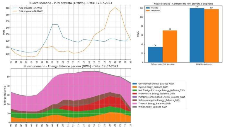
You have identified two case studies. In the first, you consider the hourly energy balance, TTF and hourly PUN curve of a 2023 high PUN day, i.e., October 16, 2023. In that case, the average PUN fell by about 10 percent and the PUN max and PUN mix differential fell from 84 to 47 €/MWh. How would your analysis change in a different context with a lower average PUN (thus low demand)?

Interesting question, related, however, to a scenario that I have not yet simulated and would prefer to feed later into the new, smarter CNN model I mentioned earlier, as soon as it is trialed and validated.

What would happen on days with less PV? Would the effect be more limited?

According to initial simulations with the experimental CNN, it would appear that on days with less sunshine, and therefore less PV, the peak shaving and valley filling effect of the production time lag associated with PV+BESS would be less pronounced.

Thus, we understood that the average BESS should decrease, and so should the maximum BESS. But what are the effects of BESS on the minimum PUN?

I specify that the average PUN would appear to decrease on the autumn-type day, thus less irradiated, while it would rise slightly on the summer-type day, which is sunnier. The minimum PUN (we always refer to the daytime one) would appear to undergo a “valley filling” effect, thus bullish. Keep in mind that the model has as a framework condition that, in the System Marginal Price governing the Day-Ahead Market, the marginal technology remains predominantly or always gas-fired. In fact, given the same scenario, if we force an increase in the TTF of the day into the model, the curves “shift” upward almost in parallel.

At the same time, we are in a historical phase of PUN overshoot. Would these analyses be valid for zonal prices as well? What is required to do such an exercise, even at the zonal level?

I would have liked to perform this study on a single market area from the outset, and it should certainly be performed preferably on a zonal basis. Unfortunately, however, I did not find the volume and level of detail of data necessary for a zonal analysis, with particular reference to the lack of availability of hourly zonal energy balances broken down by source. Therefore I had to use a more “macro” approach, in which I considered the Italian electricity system as a “black box” with as input a set of variables (or “features” in machine/deep learning jargon) and as output the PUN value. Inside this black box, I placed the CNN neural network to be properly educated, based on the hourly history of past energy balances and stock prices on a national basis. Instead, the zonal exercise would require detailed hourly energy balances, but at a zonal-specific level. The icing on the cake would be to also have hourly zonal energy balances from 2009-2010 because then CNN could be taught how the individual zone’s electricity market reacted in detail during a phase of strong PV deployment, but even these Big Data are not readily available.

Could you explain how you used deep learning techniques? Could you explain the tools you used?

For the ETL phase, which was necessary for the training and testing of the CNN, I took the historical hourly stock market data in Excel format from the “statistics” section of the GME website, the hourly national balance sheet data by source in Json format through the API made available from Terna’s developer portal, and the daily TTF spot gas quotation data on Excel from a paid platform to which we subscribe. I cleaned and merged them and used them for training and validation testing of a convolutional neural network, with three convolutional layers, three MaxPooling layers, and two “dense” layers, whose “tuning” of the so-called “hyperparameters” was performed with the valuable Hyperopt algorithm.

I also adopted “dropout” techniques to avoid the phenomenon of overfitting in the training phase, that is, to prevent the neural network from being “overtrained” and modeling the historical dataset too faithfully but then producing poor prediction results when used to predict completely new scenarios. To program it all I used only open-source software: self-written code with Python with Tensorflow libraries for deep learning, using Microsoft’s Visual Studio Code and Chat GPT 3.5 programming tips. The trigger for the need to evolve in these studies is to try to forecast the future directions of the national electricity market: having to manage the energy procurement portfolio management of the companies in our Unionenergia Consortium over long future contract horizons, “what if” analyses and forecasting activities are crucial and sometimes, as in this case, generate interesting “by-products” for other sectors as well.

So, to simplify, does it make economic sense to install BESS coupled with PV utility scale?

If the simulations I have run prove to be true in the future it would appear that the estimation of the economic viability of pairing a BESS with a PV utility scale is affected by a strong “nonlinearity” of the problem, because the higher revenue that BESS is expected to bring to the investor in terms of the daytime PUNmax – PUNmin spread, is affected by elements of uncertainty and randomness whose “magnitude” itself depends on the market spread of the BESSes themselves, which impacts the shape of the PUN curve and the cost of investing in the BESSes. A general answer to your question cannot be given: it is not easy and perhaps does not exist. They are, in fact, systems that require a cost-benefit analysis conducted with a lot of expertise and attention, implementing a careful sensitivity analysis on the variables of investment cost, the largest achievable spread and its duration, and, last but not least, the price of gas, as thermal technology will remain the marginal one in the market for a long time to come and position the level of the price curves.

Does it make sense then to say that there is an advantage for first movers? In general, does it mean that the economic sense of installing BESS combined with PV depends on the performance of the BESS market itself? So, the more there are, the less incentive there will be to install more of them?

First movers will perhaps find higher investment costs than late movers, but initially more substantial benefits than the latter. This is at least a common sense consideration in general. But then, as I mentioned earlier, much will depend on the specific zonal market production mix and the shapes of the zonal-specific price curves in which the plants are to be built. The impacts of any constraints related to the permissible configurations of the Production Units (BESS + PV behind a single Production Unit or as separate Production Units?) will also have to be checked, which, in all honesty, I do not know about and which have to be carefully evaluated according to current standards and rules. Regarding incentives, it would be inferred that their magnitude and duration will probably be a relevant element to help investors overcome any uncertainties related to the aforementioned nonlinearity of the cost-benefit analysis of these systems.

How might this inform incentives?

Regarding incentives, it would be inferred that their magnitude and duration is likely to be a relevant element to help investors overcome any uncertainties related to the aforementioned nonlinearity of the cost-benefit analysis of these systems